 First Steps in R
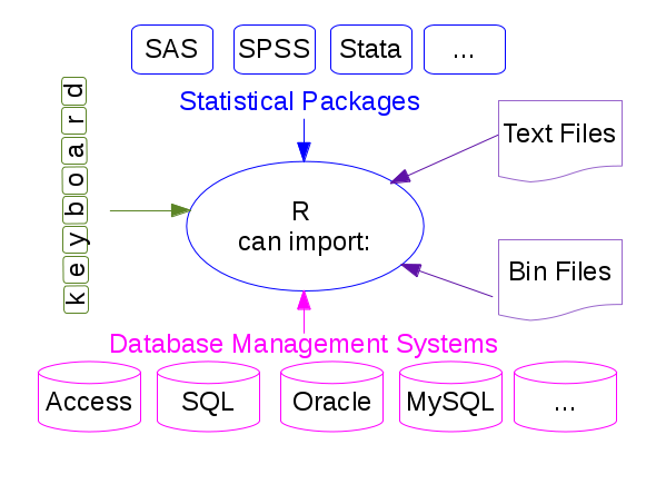
You can import data in R in many different formats!
The main functions used in R to import data from ASCII files are read.table and read.csv to read data in a tabular form, and readLines to read lines from a text file. The only difference between read.table and read.csv is that in the later the default separator is a comma. The analogous functions to write data to a text file are called write.table, write.csv, writeLines,...
Let’s have a file named galaxies.dat which contains:
GALAXY morf T.RC3 U-B B-V
NGC1357 Sab 2    0.25 0.87
NGC1832 Sb  4   -0.01 0.63
NGC2276 Sc  5   -0.09 0.52
NGC3245 S0 -2    0.47 0.91
NGC3379 E  -5    0.53 0.96
NGC1234 Sab 3   -0.56 0.84
NGC5678 E  -4    0.45 0.92
This file can be read as follows:
> gal <- read.table("galaxies.dat",header=TRUE)
where the instruction header=TRUE specifies that the first line in the file does not contain data but it is a label identifying the contents of every column.
> gal                                 # show content of data file
   GALAXY morf T.RC3   U.B  B.V       # 'U-B' and 'B-V' labels have changed!
1 NGC1357  Sab     2  0.25 0.87
2 NGC1832   Sb     4 -0.01 0.63
3 NGC2276   Sc     5 -0.09 0.52
4 NGC3245   S0    -2  0.47 0.91
5 NGC3379    E    -5  0.53 0.96
6 NGC1234  Sab     3 -0.56 0.84
7 NGC5678    E    -4  0.45 0.92
The data file is read as a data frame (i.e. a list):
> class(gal)
[1] "data.frame"
> names(gal)
[1] "GALAXY" "morf"   "T.RC3"  "U.B"    "B.V"


> gal$morf                            # text chains are read as factors
[1] Sab Sb  Sc  S0  E
Levels: E S0 Sab Sb Sc

> options(stringsAsFactors = FALSE)   # unless default behaviour is disabled
> gal <- read.table("galaxies.dat",header=TRUE)
> gal$morf
[1] "Sab" "Sb"  "Sc"  "S0"  "E"


> tapply(gal$U.B,gal$morf,mean)       # calculate mean colours for every morph. type
    E     S0    Sab     Sb     Sc
0.490  0.470 -0.155 -0.010 -0.090
The names of the different fields can be directly accessed (without lists name specification) using their names:
> attach(gal)                         # direct access to the list elements
> morf                                #   (it is no longer necessary to use gal$morf,...)
  [1] Sab Sb  Sc  S0  E
  Levels: E S0 Sab Sb Sc

> detach(gal)                         # remove direct access
If the data file only contains numbers, information can also be read and assigned to a matrix instead of storing it in a data frame. As an example, if we want to read a file with 3 columns:
> a <- matrix(data=scan("numbers.dat",0),ncol=3,byrow=TRUE)
Read 36 items
> a
      [,1]  [,2] [,3]
 [1,]    2  0.25 0.87
 [2,]    4 -0.01 0.63
 [3,]    5 -0.09 0.52
 [4,]   -2  0.47 0.91
 [5,]   -5  0.53 0.96
 [6,]    1  0.45 0.92
 [7,]    3  0.20 0.73
 [8,]   -3  0.51 0.94
 [9,]   -5  0.55 0.96
[10,]   10 -0.22 0.39
[11,]   -1  0.38 0.85
[12,]    5 -0.03 0.63
If the number of columns is not specified through ncol, all the elements are stored into a one dimensional array:
> a1 <- matrix(data=scan("numbers.dat",0))
Read 36 items
> a1
       [,1]
 [1,]  2.00
 [2,]  0.25
 [3,]  0.87
 [4,]  4.00
 [5,] -0.01
 [6,]  0.63
 [7,]  5.00
 [8,] -0.09
 [9,]  0.52
  .     .
  .     .
  .     .
[28,] 10.00
[29,] -0.22
[30,]  0.39
[31,] -1.00
[32,]  0.38
[33,]  0.85
[34,]  5.00
[35,] -0.03
[36,]  0.63
If byrow=TRUE is omitted the element assignment does not preserve the columns information:
> a2 <- matrix(data=scan("numbers.dat",0),ncol=3)
Read 36 items
> a2
       [,1]  [,2]  [,3]
 [1,]  2.00 -5.00 -5.00
 [2,]  0.25  0.53  0.55
 [3,]  0.87  0.96  0.96
 [4,]  4.00  1.00 10.00
 [5,] -0.01  0.45 -0.22
 [6,]  0.63  0.92  0.39
 [7,]  5.00  3.00 -1.00
 [8,] -0.09  0.20  0.38
 [9,]  0.52  0.73  0.85
[10,] -2.00 -3.00  5.00
[11,]  0.47  0.51 -0.03
[12,]  0.91  0.94  0.63
Note
Reading large datafiles requires a careful setting of the read.table parameters. Specifying the “colClasses” argument can make the data reading twice as fast while setting the “nrows” argument helps with the memory usage.
R contains a lot of example data. All the functions and data blocks are stored in packages.
The list of packages currently installed in R can be seen with:
> library()
Packages in library ‘/home/user/R/x86_64-redhat-linux-gnu-library/3.0’:

FITSio                  FITS (Flexible Image Transport System) utilities
manipulate              Interactive Plots for RStudio
plyr                    Tools for splitting, applying and combining  data
rstudio                 Tools and Utilities for RStudio

Packages in library ‘/usr/lib64/R/library’:

base                    The R Base Package
bitops                  Functions for Bitwise operations
boot                    Bootstrap Functions (originally by Angelo Canty for S)
class                   Functions for Classification
...
To gather information about a specific package:
> library(help=splines)               # show help about the 'splines' package

              Information on package ‘splines’

Description:

Package:       splines
Version:       3.0.1
Priority:      base
Imports:       graphics, stats
Title:         Regression Spline Functions and Classes
Author:        Douglas M. Bates <bates@stat.wisc.edu> and William N.
               Venables <Bill.Venables@csiro.au>
Maintainer:    R Core Team <R-core@r-project.org>
Description:   Regression spline functions and classes
...
And to load a package and be able to use its functionality:
> library(splines) # load 'splines' package
We can check the data lists that are currently available:
> data()
Data sets in package ‘datasets’:

AirPassengers           Monthly Airline Passenger Numbers 1949-1960
BJsales                 Sales Data with Leading Indicator
BJsales.lead (BJsales)  Sales Data with Leading Indicator
BOD                     Biochemical Oxygen Demand
CO2                     Carbon Dioxide Uptake in Grass Plants
ChickWeight             Weight versus age of chicks on different diets
DNase                   Elisa assay of DNase
EuStockMarkets          Daily Closing Prices of Major European Stock
...
And those that are available in a given package:
> data(package="cluster")             # show data available through the package 'cluster'

Data sets in package ‘cluster’:

agriculture             European Union Agricultural Workforces
animals                 Attributes of Animals
chorSub                 Subset of C-horizon of Kola Data
flower                  Flower Characteristics
plantTraits             Plant Species Traits Data
...

> data(animals,package="cluster")     # load 'animals' list from 'cluster' package
One of the strongest points in R is that new packages are continuously being generated, including new functionalities. To install a new package:
> install.packages("car")             # install 'car' package
Installing package into ‘/home/ceballos/R/x86_64-redhat-linux-gnu-library/3.0’
...

--- Please select a CRAN mirror for use in this session ---  # ask for a software mirror
Once installed we can use it:
> library(car)                        # load in memory the functionality defined in 'car'
> data(package="cluster")
Data sets in package ’car’:

AMSsurvey                     American Math Society Survey Data
Adler                         Experimenter Expectations
...